
Common cases that the GRM doesn’t invert
Published:
Here, I show common genetic reasons where can lead to genomic relationship matrix (GRM) with problems in the inversion. They are commonly based on population structure or repeated (or highly similar) information. The cases are not always true, but they can represent why you have a strong linear dependence in your G matrix (Van Raden 2008) and a not unique inverse for the matrix. After identifying the reason, you can take action in order to manage the data before building the G matrix.
If you know any other common reason, please let me know and I can add it to the list. :)
Data used are real and from freely available data sets from BGLR R package and AGHmatrix.
library(AGHmatrix) #for potato and pine data set and G functions
library(BGLR) #for wheat data set
library(ggfortify) #for PCAs
## Loading required package: ggplot2
G matrix with determinant higher than 0
An example of an invertable G matrix, the data set has no repeated individuals, no apparent population structure, and way more markers than individuals.
data(snp.sol)
dim(snp.sol)
## [1] 571 3895
G_OK <- Gmatrix(snp.sol, ploidy=4)
## Initial data:
##  Number of Individuals: 571
##  Number of Markers: 3895
##
## Missing data check:
##  Total SNPs: 3895
##   0 SNPs dropped due to missing data threshold of 1
##  Total of: 3895  SNPs
## MAF check:
##  No SNPs with MAF below 0
## Monomorphic check:
##  No monomorphic SNPs
## Summary check:
##  Initial:  3895 SNPs
##  Final:  3895  SNPs ( 0  SNPs removed)
##
## Completed! Time = 2.245  seconds
det(G_OK)
## [1] -5.523282e-288
G_OK_Inv <- solve(G_OK)
PCs <- prcomp(G_OK, scale=TRUE)
autoplot(PCs)
1) Repeated individuals
I repeat the first line in snp.sol (as a clone or repeated individual), notice the off-diagonal value close to 1 in this case.
snp.sol1 <- rbind(snp.sol[1,],snp.sol)
G1 <- Gmatrix(snp.sol1, ploidy=4)
## Initial data:
##  Number of Individuals: 572
##  Number of Markers: 3895
##
## Missing data check:
##  Total SNPs: 3895
##   0 SNPs dropped due to missing data threshold of 1
##  Total of: 3895  SNPs
## MAF check:
##  No SNPs with MAF below 0
## Monomorphic check:
##  No monomorphic SNPs
## Summary check:
##  Initial:  3895 SNPs
##  Final:  3895  SNPs ( 0  SNPs removed)
##
## Completed! Time = 2.06  seconds
det(G1)
## [1] 0
#G1_Inv <- solve(G1) #error!
G1[1:4,1:4] #off-diagonal values close to 1
##                       MSH228-6  Manistee   MSS297-3
##          1.00038749 1.00038749 0.1536395 0.09283224
## MSH228-6 1.00038749 1.00038749 0.1536395 0.09283224
## Manistee 0.15363950 0.15363950 0.9382326 0.15281292
## MSS297-3 0.09283224 0.09283224 0.1528129 1.03410691
2) Highly related individuals
I repeat the first line in snp.sol and add some noise to it, (as a fullsib or some highly related pair of individuals). Often you can have an “inverse” but it has numeric problems like here:
snp.high.rel <- snp.sol[1,]
snp.high.rel <- snp.high.rel + sample(c(-1,0,1),3895,replace=TRUE)
snp.high.rel <- ifelse(snp.high.rel<0,0,snp.high.rel)
snp.high.rel <- ifelse(snp.high.rel>4,4,snp.high.rel)
snp.sol1 <- rbind(snp.high.rel,snp.sol)
G1 <- Gmatrix(snp.sol1, ploidy=4)
## Initial data:
##  Number of Individuals: 572
##  Number of Markers: 3895
##
## Missing data check:
##  Total SNPs: 3895
##   0 SNPs dropped due to missing data threshold of 1
##  Total of: 3895  SNPs
## MAF check:
##  No SNPs with MAF below 0
## Monomorphic check:
##  No monomorphic SNPs
## Summary check:
##  Initial:  3895 SNPs
##  Final:  3895  SNPs ( 0  SNPs removed)
##
## Completed! Time = 2.199  seconds
G1[1:4,1:4] #high relationship
##              snp.high.rel   MSH228-6  Manistee   MSS297-3
## snp.high.rel   1.51519434 0.86777224 0.1150521 0.06966883
## MSH228-6       0.86777224 0.99994213 0.1537969 0.09301776
## Manistee       0.11505209 0.15379691 0.9375168 0.15278083
## MSS297-3       0.06966883 0.09301776 0.1527808 1.03325055
det(G1) #you can get a determinant
## [1] 2.651697e-288
G1_Inv <- solve(G1) #you can get a invert
G1_Inv[1:4,1:5] #but it has numerical issues
##              snp.high.rel    MSH228-6    Manistee    MSS297-3       NY156
## snp.high.rel  27313010512 27313010509 27313010511 27313010511 27313010511
## MSH228-6      27313010509 27313010521 27313010510 27313010510 27313010511
## Manistee      27313010511 27313010510 27313010521 27313010511 27313010511
## MSS297-3      27313010511 27313010510 27313010511 27313010515 27313010511
3) More individuals than markers
I subset the snp.sol letting it with just 500 markers and all the 571 individuals.
snp.sol2 <- snp.sol[,1:500]
G2 <- Gmatrix(snp.sol2, ploidy=4)
## Initial data:
##  Number of Individuals: 571
##  Number of Markers: 500
##
## Missing data check:
##  Total SNPs: 500
##   0 SNPs dropped due to missing data threshold of 1
##  Total of: 500  SNPs
## MAF check:
##  No SNPs with MAF below 0
## Monomorphic check:
##  No monomorphic SNPs
## Summary check:
##  Initial:  500 SNPs
##  Final:  500  SNPs ( 0  SNPs removed)
##
## Completed! Time = 0.169  seconds
det(G2)
## [1] 0
#G2_Inv <- solve(G2) #error!
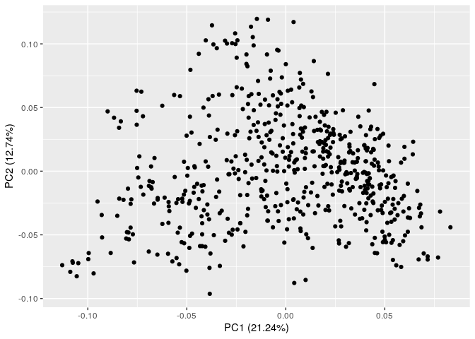
4) Population Structure
wheat data set has a population structure with 2 subpopulations.
data(wheat)
dim(wheat.X)
## [1] 599 1279
G3 <- Gmatrix(wheat.X, ploidy=2)
## Initial data:
##  Number of Individuals: 599
##  Number of Markers: 1279
##
## Missing data check:
##  Total SNPs: 1279
##   0 SNPs dropped due to missing data threshold of 1
##  Total of: 1279  SNPs
## MAF check:
##  No SNPs with MAF below 0
## Monomorphic check:
##  No monomorphic SNPs
## Summary check:
##  Initial:  1279 SNPs
##  Final:  1279  SNPs ( 0  SNPs removed)
##
## Completed! Time = 0.62  seconds
det(G3)
## [1] 0
#G3_Inv <- solve(G3) #error!
PCs <- prcomp(G3, scale=TRUE)
autoplot(PCs)
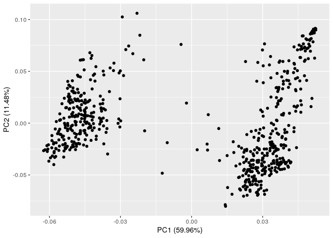
5) Population structure at the family level
snp.pine data set has a population structure at the family level (each cluster in the PCA).
data(snp.pine)
dim(snp.pine)
## [1] 926 4853
G4 <- Gmatrix(snp.pine, ploidy=2)
## Initial data:
##  Number of Individuals: 926
##  Number of Markers: 4853
##
## Missing data check:
##  Total SNPs: 4853
##   0 SNPs dropped due to missing data threshold of 1
##  Total of: 4853  SNPs
## MAF check:
##  No SNPs with MAF below 0
## Monomorphic check:
##  No monomorphic SNPs
## Summary check:
##  Initial:  4853 SNPs
##  Final:  4853  SNPs ( 0  SNPs removed)
##
## Completed! Time = 5.838  seconds
det(G4)
## [1] 0
#G4_Inv <- solve(G4) #error!
PCs <- prcomp(G4, scale=TRUE)
autoplot(PCs)

References for packages and data sets
citation("AGHmatrix")
citation("BGLR")
citation("ggfortify")
Amadeu, R. R., C. Cellon, J. W. Olmstead, A. A. F. Garcia, M. F. R. Resende, and P. R. Muñoz. 2016. AGHmatrix: R Package to Construct Relationship Matrices for Autotetraploid and Diploid Species: A Blueberry Example. The Plant Genome 9.
Perez, P., and de los Campos, G., 2014 Genome-Wide Regression and Prediction with the BGLR Statistical Package. Genetics 198 (2): 483-495.
VanRaden, P.M., 2008. Efficient methods to compute genomic predictions. Journal of dairy science, 91(11), pp.4414-4423.
Yuan Tang, Masaaki Horikoshi, and Wenxuan Li. ggfortify: Unified Interface to Visualize Statistical Result of Popular R Packages. The R Journal 8.2 (2016): 478-489.